Aplicativo GNUPLOT / GNUPLOT Tutorial

Aplicativo GNUPLOT / GNUPLOT software

Comandos básicos, tutorial e exemplos de aplicação
Basic commands, tutorial, and application examples

Página inicial / Home
Página Oficial (www.gnuplot.info)

Exemplos: 1, 2, 3, 4, 5, 6.
Download

A TERRA EM DIFERENTES PROJEÇÕES CARTOGRÁFICAS
THE EARTH IN DIFFERENT MAP PROJECTIONS
Exemplos - Página 1

Uma interessante aplicação do GNUPLOT é na visualização de Projeções Cartográficas, podendo ser útil no aprendizado de Cartografia Matemática, uma vez que o aluno pode escrever as equações das projeções, modificar o paralelo padrão, modificar o ponto de tangência, modificar a escala, calcular o fator de escala, visualizar a projeção, dentre outras possibilidades.

Na sequência são apresentadas algumas projeções, acompanhadas dos respectivos scripts.

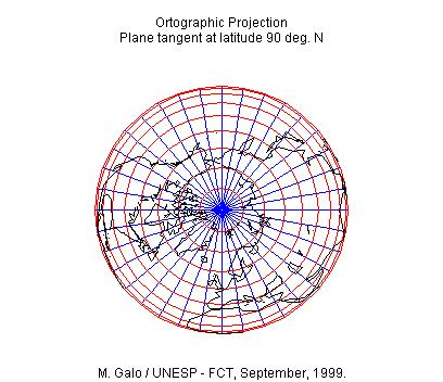
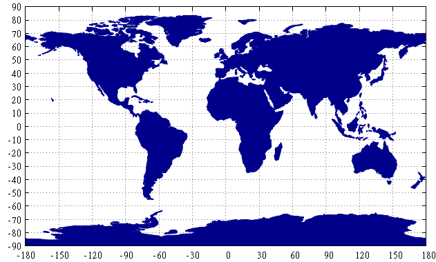
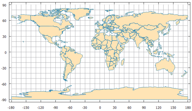
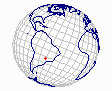
Projeção Plana Ortográfica com o plano tangente na latitude 90^o N

# ---------------------------------
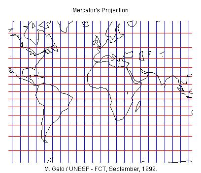
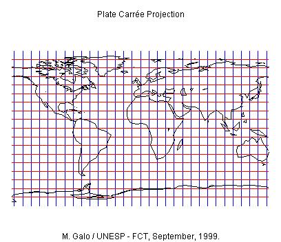
# Ortographic Projection
#
# Author: Eng. Cart. Mauricio Galo
# UNESP/Department of Cartography
# Sep./1999, 2016
#
reset
set noxtics
set noytics
set angles degrees
set nogrid
set noborder
width=40
height=width*(3./4.)
set xrange [-width : width]
set yrange [-height : height]
set title "Ortographic Projection\n\
Plane tangent at latitude 90 deg. N"
ap=25
lat0=90
lon0=0
delta_lat=90
delta_lon=180
l_sup=lat0+delta_lat
l_inf=lat0-delta_lat
l_esq=lon0-delta_lon
l_dir=lon0+delta_lon
X(lat,lon)=ap*(cos(lat0)*sin(lat)-sin(lat0)*cos(lat)*cos(lon-lon0))
Y(lat,lon)=ap*cos(lat)*sin(lon-lon0)
XC(lat,lon)= (lat >=l_inf && lat <=l_sup) ? X(lat,lon) : 0/0
YC(lat,lon)= (lon >=l_esq && lon <=l_dir) ? Y(lat,lon) : 0/0
plot 'world.mer' using (YC($2,$1)):(XC($2,$1)) t '' with lines lc 3
rep 'world.par' using (YC($2,$1)):(XC($2,$1)) t '' with lines lc 1
rep 'world.dat' using (YC($2,$1)):(XC($2,$1)) t '' with lines lc 8
pause -1 "Continua?"

Projeção Plana Ortográfica com o plano tangente na latitude 90^o S

# ----------------------
# Ortographic Projection
#
reset
set noxtics
set noytics
set angles degrees
set nogrid
set noborder
width=40
height=width*(3./4.)
set xrange [-width : width]
set yrange [-height : height]
set title "Ortographic Projection\n\
Plane tangent at latitude 90 deg. S"
ap=25
lat0=-90
lon0=0
delta_lat=90
delta_lon=180
l_sup=lat0+delta_lat
l_inf=lat0-delta_lat
l_esq=lon0-delta_lon
l_dir=lon0+delta_lon
X(lat,lon)=ap*(cos(lat0)*sin(lat)-sin(lat0)*cos(lat)*cos(lon-lon0))
Y(lat,lon)=ap*cos(lat)*sin(lon-lon0)
XC(lat,lon)= (lat >=l_inf && lat <=l_sup) ? X(lat,lon) : 0/0
YC(lat,lon)= (lon >=l_esq && lon <=l_dir) ? Y(lat,lon) : 0/0
plot 'world.mer' using (YC($2,$1)):(XC($2,$1)) t '' with lines lc 3
rep 'world.par' using (YC($2,$1)):(XC($2,$1)) t '' with lines lc 1
rep 'world.dat' using (YC($2,$1)):(XC($2,$1)) t '' with lines lc 8
pause -1 "Continua?"

Projeção Plana Ortográfica modalidade equatorial (Plano tangente no Equador)

# ----------------------
# Ortographic Projection
#
reset
set noxtics
set noytics
set angles degrees
set nogrid
set noborder
width=40
height=width*(3./4.)
set xrange [-width : width]
set yrange [-height : height]
set title "Ortographic Projection\n\
Plane tangent on the Equator"
ap=25
lat0=0
lon0=-30
delta_lat=90
delta_lon=90
l_sup=lat0+delta_lat
l_inf=lat0-delta_lat
l_esq=lon0-delta_lon
l_dir=lon0+delta_lon
X(lat,lon)=ap*(cos(lat0)*sin(lat)-sin(lat0)*cos(lat)*cos(lon-lon0))
Y(lat,lon)=ap*cos(lat)*sin(lon-lon0)
XC(lat,lon)= (lat >=l_inf && lat <=l_sup) ? X(lat,lon) : 0/0
YC(lat,lon)= (lon >=l_esq && lon <=l_dir) ? Y(lat,lon) : 0/0
plot 'world.mer' using (YC($2,$1)):(XC($2,$1)) t '' with lines lc 3
rep 'world.par' using (YC($2,$1)):(XC($2,$1)) t '' with lines lc 1
rep 'world.dat' using (YC($2,$1)):(XC($2,$1)) t '' with lines lc 8
pause -1 "Continua?"

Projeção Plana Estereográfica modalidade equatorial

# ----------------------------------
# Estereographic Azimutal Projection
#
reset
set noxtics
set noytics
set angles degrees
set nogrid
set noborder
width=40
height=width*(3./4.)
set xrange [-width : width]
set yrange [-height : height]
set title "Estereographic Azimutal Projection"
ap=10
lat0=0
long0=0
den(lat,lon)=1+sin(lat0)*sin(lat)+cos(lat0)*cos(lat)*cos(lon-long0)
XC(lat,lon)=2*ap*( cos(lat0)*sin(lat)-\
sin(lat0)*cos(lat)*cos(lon-long0) )/den(lat,lon)
YC(lat,lon)=2*ap*cos(lat)*sin(lon-long0)/den(lat,lon)
plot 'world.mer' using (YC($2,$1)):(XC($2,$1)) t '' with lines lc 3
rep 'world.par' using (YC($2,$1)):(XC($2,$1)) t '' with lines lc 1
rep 'world.dat' using (YC($2,$1)):(XC($2,$1)) t '' with lines lc 8
pause -1 "Continua?"

Projeção de Mercator

# ---------------------
# Mercator's Projection
#
reset
set noxtics
set noytics
set angles degrees
set nogrid
set noborder
width=40
height=width*(3./4.)
set xrange [-width : width]
set yrange [-height : height]
drad=pi/180.
set title "Mercator's Projection"
# Semi-axis of the model
r=20
# Longitude of the central meridian (degrees)
long0=0
# Internatioal Elipsoid, adopted by IUGG in 1967: a=6378160 f=1/298.25
# f=(a-b)/a
# e2=1-(1-f)**2
# Obs.: The use of elipsoid of revolutions is not necessary in this
# scale and It`s only used as a example.
a=6378160.0
inv_f=298.25
f=1/inv_f
e2=1-(1-f)**2
e=sqrt(e2)
# Semi-major axis (a) of the model on the projection: ap
ap=r
T(lat)=tan(45+lat/2)*( (1-e*sin(lat))/(1+e*sin(lat))**(e/2) )
XC(lat,lon)=ap*log(T(lat))
YC(lat,lon)=ap*(lon-long0)*drad
plot 'world.mer' using (YC($2,$1)):(XC($2,$1)) t '' with lines lc 3
rep 'world.par' using (YC($2,$1)):(XC($2,$1)) t '' with lines lc 1
rep 'world.dat' using (YC($2,$1)):(XC($2,$1)) t '' with lines lc 8
pause -1 "Continua?"

Projeção "Plate-Carrée" ou Projeção Equirretangular ou
Projeção Cilíndrica Equidistante Meridiana ou "Plane Chart"

# -----------------------
# Plate-Carrée Projection
#
reset
set noxtics
set noytics
set angles degrees
set nogrid
set noborder
width=40
height=width*(3./4.)
set xrange [-width : width]
set yrange [-height : height]
drad=pi/180.
set title "Plate Carrée Projection"
ap=15
long0=0
XC(lat,lon)=ap*lat*drad
YC(lat,lon)=(lon-long0)*ap*drad
plot 'world.mer' using (YC($2,$1)):(XC($2,$1)) t '' with lines lc 3
rep 'world.par' using (YC($2,$1)):(XC($2,$1)) t '' with lines lc 1
rep 'world.dat' using (YC($2,$1)):(XC($2,$1)) t '' with lines lc 8
pause -1 "Continua?"

Projeção Cilíndrica Equivalente de Lambert

# ---------------------------------
# Cilindrical Equivalent Projection
#
reset
set noxtics
set noytics
set angles degrees
set nogrid
set noborder
width=40
height=width*(3./4.)
set xrange [-width : width]
set yrange [-height : height]
drad=pi/180.
set title "Cylindrical Equivalent Projection\n\
(Lambert Cylindrical Equivalent Projection)"
ap=15
long0=0
XC(lat,lon)=ap*sin(lat)
YC(lat,lon)=(lon-long0)*ap*drad
plot 'world.mer' using (YC($2,$1)):(XC($2,$1)) t '' with lines lc 3
rep 'world.par' using (YC($2,$1)):(XC($2,$1)) t '' with lines lc 1
rep 'world.dat' using (YC($2,$1)):(XC($2,$1)) t '' with lines lc 8
pause -1 "Continua?"

Projeção Equivalente de Sanson-Flamsteed

# --------------------------------------
# Sanson-Flamsteed Equivalent Projection
#
reset
set noxtics
set noytics
set angles degrees
set nogrid
set noborder
width=40
height=width*(3./4.)
set xrange [-width : width]
set yrange [-height : height]
drad=pi/180.
set title "Sanson-Flamsteed Equivalent Projection"
ap=12
long0=0
XC(lat,lon)=ap*lat*drad
YC(lat,lon)=(lon-long0)*ap*cos(lat)*drad
plot 'world.mer' using (YC($2,$1)):(XC($2,$1)) t '' with lines lc 3
rep 'world.par' using (YC($2,$1)):(XC($2,$1)) t '' with lines lc 1
rep 'world.dat' using (YC($2,$1)):(XC($2,$1)) t '' with lines lc 8
pause -1 "Continua?"

Projeção Azimutal Equidistânte - Caso Polar

Projeção utilizada no emblema das Nações Unidas (UN)

# -------------------------------------------------------------------
# Projeção Azimutal Equidistante - Caso Polar
# Autor: M. Galo, UNESP / Dep. de Cartografia
#
# Projeção utilizada no emblema das Nações Unidas (UN)
# Referência para as equações da projeção: Snyder (1987, p. 195)
#
# Snyder, J. P. Map Projection - A Working Manual. U. S. Geological
# Survey Professional Paper 1395. United States Government Printing
# Office, Washington, 1987.
#

reset
unset mouse
set noxtics
set noytics
set angles degrees
set nogrid
set noborder
set size square

lon0 = 0
r = 1
LIMequid = 150

dlon(lon)=lon-lon0
xeq(lat,lon)=r*(pi/2 - lat*pi/180)*sin(dlon(lon))
yeq(lat,lon)=-r*(pi/2 - lat*pi/180)*cos(dlon(lon))

dist(lat)=abs(lat-90)

xequid(lat,lon) = ( dist(lat) <= LIMequid ) ? xeq(lat,lon) : 1/0
yequid(lat,lon) = ( dist(lat) <= LIMequid ) ? yeq(lat,lon) : 1/0

plot 'world.par' using (xequid($2,$1)):(yequid($2,$1)) t'' with lines lc 9
rep 'world.mer' using (xequid($2,$1)):(yequid($2,$1)) t'' with lines lc 9
rep 'worldn.dat' using (xequid($2,$1)):(yequid($2,$1)) with filledcurve t"" fs solid 1.0 lc rgb 'dark-blue'
pause -1 "Fechar"

Projeção Cônica Equivalente de Albers
(Paralelo Padrão na latitude 20^o S)

Projeção Cônica Equivalente de Albers
(Paralelo Padrão na latitude 20^o N)

Projeção Cônica Conforme de Lambert
Origem: (Longitude, Latitude)=(54^o O, 20^o S)

Projeção de Eckert I

Projeção de Eckert II

Propriedade principal: preserva as áreas (equivalente)

Projeção de Eckert III

Projeção de Eckert V

Projeção Equivalente de Wagner VII ou
Hammer-Wagner

Projeção Equivalente de Werner

Pequeno Globo / Small Globe - GIF animado criado a partir de uma sequência de imagens com o globo na Projeção Plana Ortográfica. As imagens foram geradas a partir de diferentes pontos de tangência localizados sobre o equador.

Arquivos de dados.

Em todas as projeções mostradas nesta página, três arquivos vetoriais foram utilizados, conforme a descrição abaixo:

- world.dat - Arquivo ASCII com as coordenadas (longitude,latitude) dos pontos que delimitam os contornos dos continentes. Este arquivo acompanha o GNUPLOT e se localiza no sub-diretório demo.
- world.par - Arquivo ASCII com as coordenadas (longitude,latitude) dos pontos que determinam os paralelos, considerando uma equidistância de 10^o.
- world.mer - Arquivo ASCII com as coordenadas (longitude,latitude) dos pontos que determinam os meridianos, considerando uma equidistância de 10^o.

O arquivo compactado dados_world.zip contém todos os três arquivos descritos.

Referências

[1] BAKKER, M. P. R. de Cartografia - Noções Básicas. Rio de Janeiro: Diretoria de Hidrografia e Navegação, 1965.
[2] BUGAYEVSKIY, L. M.; SNYDER, J. P. Map Projections - A reference Manual. London: Taylor & Francis, 1995.
[3] RICHARDUS, P.; ADLER, R. K. Map Projections for Geodesists, Cartographers and Geographers. Amsterdam: North-Holland Publishing Company, 1974. 174p.
[4] SNYDER, J. P. Map Projections - A Working Manual. Washington: United States Government Printing Office, 1987. U. S. Geological Survey Professional Paper 1395.
[5] SNYDER, J. P. Flattening the Earth: Two Thousand Years of Map Projections. Chicago: The University of Chicago Press, 1993.

Autor: Mauricio Galo, UNESP, Departamento de Cartografia
Presidente Prudente - SP